The contemporary human environment is mostly urban. We have been living in cities for millennia, which came hand in hand with phenomena inherent to humanity, such as knowledge sharing, transport or defensive efficiency. The process of forming cities occurred following a mixture of natural conditions, self-organisation mechanics and a bit of unpredictability. All these lie in the scope of research for historians and urban planners. The above factors are almost impossible to generalise as the mechanics vary between cultures, historical moments and individual approaches.

When working on adrift, I could only take some nuances into account. I will present below a few observations I made while designing the piece.

Terrain

The process that determines almost all algorithmic decisions is terrain generation. Yet, it is the only substantial aspect of the code entirely driven by pseudorandom values. The terraforming is divided into three phases: noise map generation, erosion and establishing water level.

First, the algorithm generates an empty map: a two-dimensional array filled with numbers defined and modified with a noise function applied multiple times. Different noise scales and the possibility to truncate the values affect big masses of land and sea, highlands, mountain chains, hills and a general undulation.

The second terraforming factor is the erosion function. It mimics the process of removing and depositing masses of terrain by simulating the flow of water droplets. Each droplet starts as a random point on the map, and, during hundreds of iterations, it shifts towards lower places. The height of the terrain the drop moves through is decreased or increased by an amount determined by the corrosiveness of the zone, the speed of the drop, and its size. This process is repeated thousands of times to simulate the flow of large volumes of water, ensuring that the results of the erosion of one drop affect the behaviour of others. Using different resolutions results in various geological formations: from primordial glacial landforms such as fiords, valleys, and moraines to small rills and gullies on the sides of mountains.

[The erosion algorithm is my javascript adaptation of Hydraulic-Erosion by Sebastian Lague (MIT License)]

Finally, the sea level is established by a random number representing the percentage of land covered with water. For example, for the value of 0.6, the map's numbers are shifted so that 60% of all the coordinates are above level zero.

Potential settlement locations

In the second phase of the process, the algorithm analyses the terrain map for its ability to host potential human settlements. To determine the criteria for such analysis, I made certain assumptions about what topographical conditions can be considered apt for locations of towns and cities. I prioritise extensive plains, mild hills and coastal areas over zones with high variability or very steep areas. These are not always necessarily true in reality, and – not to discard any possibility – I decided to give the more complex regions a slight chance to host a city. I call them wild cards, which are granted randomly.

The information about the feasibility of urban development is stored in a map (a two-dimensional array that I call the city map) of the same size as the terrain map. Each point is assigned a value of zero by default. If the feasibility assessed by the algorithm is high (e.g. it is located in a valley and the terrain is not steep or a wild card is randomly granted), then the size of the settlement is chosen. It can vary between a small town, middle-size city, large city or a metropolis. Each of these categories stands for how big an area the settlement potentially occupies, i.e. how many neighbouring points are assigned a random value larger than zero.

The potential city coordinates are stored in an array to be reused in the next phase.

Merchant routes

The road map is the third layer that determines human habitat development. It represents a major factor for cities' development throughout history: the trade routes.

I implemented a customised version of the shortest walk algorithm to establish a network of connections between potential cities. This algorithm finds the most optimal paths between pairs of points in a network. Optimal, in this case, does not necessarily mean shortest but cheapest within established criteria. For example, I consider a connection cheap if it leads from one point to another through relatively flat terrain or valleys (without climbing or descending steep hills). In contrast, an expensive connection is one that requires a traveller to climb cliffs or swim through water. If a path is once traversed, then traversing it again has a lower cost.

As a base for calculating optimal routes, I create a network of edges that mark potential connections between each point on the map and its closest neighbours. This network, or graph, is stored as a JavaScript map object. Every edge (the connection between two adjacent points) is assigned a cost of traversing it. This cost is based on the terrain map and the city map. The bigger the slope of the connection, the more expensive it is to traverse it. The cost is decreased if the edge is on potentially urban terrain. I drastically reduce the cost if it is on the coast to boost the brightness of coastal areas in the final result.

[I adapted a C# script from the article “Pathfinding Algorithms in C#” by Kristian Ekman published in Code Project licensed under The Code Project Open License (CPOL). The code was translated to javascript and simplified for performance.]

The road map is, by default, a two-dimensional array filled with zeros. Two potential city locations are chosen at random for each new connection, and the algorithm calculates the optimal path between them based on the provided network of edges and their costs. All the road map points on the way have their value increased by one, and the cost of edges connecting them is lowered.

[The above paragraph contains a simplification. Due to how the shortest walk algorithm works, I optimised the function for speed while slightly sacrificing the uniformity of the random distribution of connections. In adrift, first, one random destination point is chosen. Then, the cost of reaching the destination is calculated for all the points in the network. Finally, multiple origin points are selected randomly, and the optimal paths between the origin and destination points are recreated based on the cost calculation.]

This process is repeated hundreds of times, resulting in a map reflecting a network of road-like connections. These roads tend to be located in valleys, on coastal areas, and they avoid traversing mountainous terrains. The roads meander between the elevations in hilly zones, while they tend to be direct on plains. If crossing a very mountainous mass or water results in the cheapest alternative, such connections are usually more direct, so they are as short as possible. Some paths are visibly centralised arteries, which results from the fact that once a connection is established, the probability of reusing it is higher.

Putting things together

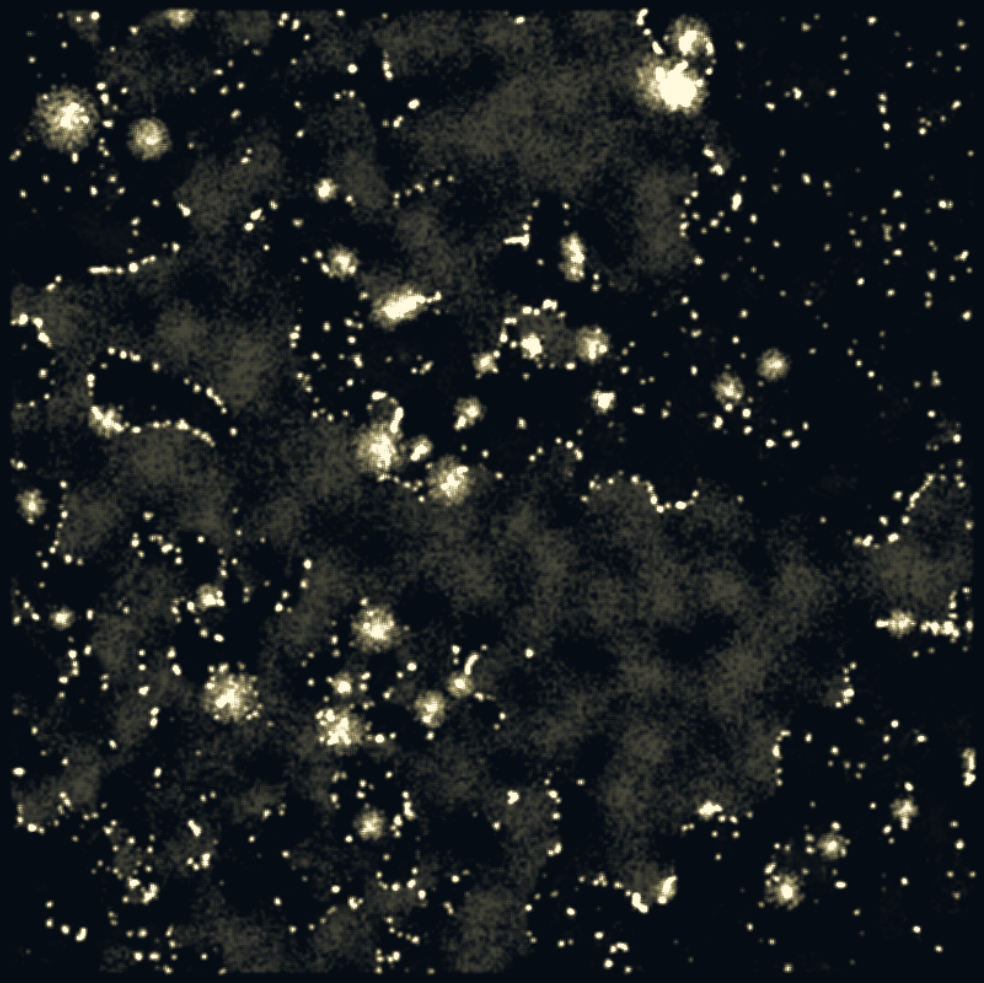
The map that is directly used for generating the images is a result of the juxtaposition of the data calculated until this point. I call this last two-dimensional array a light map. Before calculating it, a few additional arrays are computed by the algorithm. The first one is the blurred roadmap. It is the result of smoothing values from the roadmap iteratively so that what remains is a type of area of influence of the paths. The sharp lines disappear, but their vicinities – until now with values close to zero – are granted higher numbers. The second one is a sharp roadmap, which is similar to the original roadmap with minimum smoothing strength applied, only to avoid jagged geometries of the roads. Finally, blurred citymap is the result of applying the same logic as in blurred roadmap to potential cities; however, the results are different. Because of the fact that the areas of city probabilities are large, the centres of agglomerations remain almost intact, while the edges dissipate into more extensive areas of influence.

Per each point in the array, the algorithm calculates the resulting light values using the following formula, which I tweaked to achieve the best results.

//ct - blurred citymap value 
//rd - blurred roadmap value
//sm - sharp roadmap value
//NOISE - stands for the noise function

lightmap[i][j] = 3*Math.sqrt(Math.pow(ct,1.5)*Math.pow(Math.min(0.21,rd),0.75)) 
  + ((rd<0.03) ? 0 : 2.5*Math.min(0.4,Math.pow(1.2*ct,1.35))*NOISE)
  + 0.65*Math.max(0,1-ct)*rd*NOISE);
  + 0.65*sm*Math.sqrt(ct);

The general explanation is that the places where there is either no blurred city influence (values very close to zero) or blurred road influence remain dark. For a point to have a high light value, it must be located in an area with both city and road influence. Additionally, for some regions of the map (determined with a noise function), roads leave traces so that there is a visible network of connections outside towns. I also introduced a certain level of randomness to avoid homogenous bright areas.

The lightmap undergoes the process of erosion that provides it with a more realistic look. Wider stripes of light are turned into thinner, meandering crests, and cities are slightly broken into what I interpret as districts.

Other layers and technical aspects

In this article, I wanted to focus on the mechanisms behind the algorithmic simulation of human habitats at a large scale. Other elements of the outcome (atmosphere, stars, events) are important for the narrative but – in my opinion – less interesting from the point of view of the algorithmic process. Nevertheless, many follow strategies similar to the ones described above. To give an example, I will briefly explain the process of generating the layer of clouds.

Clouds - similarly to the terrain - are generated with noise function followed by the process of erosion. Certain adjustments to noise, such as applying only absolute values, give the layer the effect of different types of clouds (like altocumuli: the clouds that look like a herd of sheep). Afterwards, the map is deformed using a function that simulates vortices. Every value in the map is shifted by rotating the sample point around the centre of each vortex by a value that is proportional to its spin and inversely proportional to the distance from the centre. The function is applied recursively so that the transformation is consistent for multiple vortices.

For rendering, the algorithm distributes samples – random points on a map that store the following information: coordinates, its height calculated from the terrain map, and the light (from the light map) converted to a colour value. There are two sets of transformations that the algorithm calculates to render each sample point.

First, we need to convert the position of a point on a map to three-dimensional space, essentially inverting the process of creating a map. To do that, I assumed that the planet is perfectly spherical, and I arbitrarily set the latitude and longitude of the edges of the map to be close to the equator. Through this, I avoid major distortions of geometry.

//The below values result from multiple trials of what I considered to look best in terms of scale and deformations:
// - I set the top edge to be on the "equator" of the sphere (0 deg latitude)
// - The bottom edge is set to the latitude of around 36S (0.624 in radians)
// - The left edge's longitude is set to approx. 10E (0.168 radians)
// - The right edge's longitude is set to 10W

x = (earthRadius+height) * cos(lat+90deg) * cos(lon);
y = (earthRadius+height) * cos(lat+90deg) * sin(lon);
z = (earthRadius+height) * sin(lat+90deg);

The second transformation is projecting each point onto a plane representing the image. You can picture this process as casting rays from each sample towards a point behind the image until they intersect with the plane. This point behind the image is called a vanishing point.

The above steps are similar in other layers, but they differ by the height of the sample and the colour value. Additionally, I applied some minor tweaks to achieve the desired result.

The big picture

When we zoom out, the details get fuzzy and lose their importance both technically and metaphorically. It is not possible to include all the characteristics of human habitat in the code of a single project, and neither is describing every technical aspect of the code in a short article. I imagine it's how it feels to see the Earth from far away: we get a general grasp. The big picture.

But the details are there. I believe a good way to conclude this article is to zoom back in; to give an overview of several editions minted by collectors on fxhash and show the hidden process behind each piece.

All the images used in the article to illustrate different algorithmic processes are extracted from iterations #9 and #70. Both represent terrains with relatively balanced sea level and height variability resulting in a uniform distribution of cities of different sizes. Iteration #70 includes a few major in-land cities, while iteration #9 exhibits increased density in coastal areas (especially visible in the second plan).

The low sea level and large plains in the central part of this iteration allowed for the development of a big city that dominates the landscape located at the intersection of many major routes.

A large sea divides the landscape into two very different masses. The one on the left - broken into fiords and small islands is too difficult for connections to consolidate so that no major city can develop. The one on the right is mountainous in large part and has a long smooth coastline, which determined the location of major city visible in the second plan.

This iteration includes Aegean-like sea with a big mass of mountainous terrain in the upper part of the map. The coastline between these two formations was the best place for almost linear urbanisations to emerge.

A lot of variation of terrain: mountainous mass in the top part of the map with fiords to the right and plains at the bottom with the relatively smooth coastline. We can see linear coastal towns on the lower left side and multiple middle size cities scattered between the mountains. Surprisingly, major intersections of road networks do not coincide with bigger cities.

The route network is imbalanced and divided into two clusters: underdeveloped on the left and an entangled mix of connection on the right. The latter lead to an agglomeration of 4-5 major cities that dominate the view.

Different terrain conditions result in a wide variety of different cities - from scattered small towns, to linear developments in the coast and spits, to big cities on network intersections.

Two twin cities dominate the landscape with a few centralised routes that span from the central continent towards islands and spits in the top right, top left and right part of the map.

A mass of terrain with a zone of lakes on the left and a very visible network of connections centralised in a few major cities.

These are just a few examples. If you are curious about the process behind your iteration of adrift or any technical aspect not described in the article, feel free to contact me on twitter.