Noise() Equalization

This article outlines a technique I’ve used in my last few pieces to equalize noise() values across the canvas to obtain relatively equal counts of values between 0 and 1.

Disclaimer: I’m a self-taught coder and started with p5.js & javascript just over a year ago. I can pretty much guarantee that there’s a better way to do what I’m about to describe. At least this may serve as inspiration!

So, why might we want to do equalize noise() values?

When using noise() across the canvas with a very small scale factor, e.g. noise(x*0.0005, x * 0.0005), we obtain a smooth but very narrow distribution of values:

For example (showing only key bits of code):

squareSize = 10;
noise_scale = 0.0005;
  
for (let row = 0; row < height / squareSize; row++) {
  for (let col = 0; col < width / squareSize; col++) {
  
    let x = col * squareSize;
    let y = row * squareSize;

    n = noise(x * noise_scale, y * noise_scale);

    fill(n * 255);

    rect(x, y, squareSize, squareSize);

  }
}

A histogram of the above noise() values between 0 and 1 looks like this:

If we want to use these values to select from a list of options for a given parameter, e.g., colours from a palette, we’ll only get a narrow slice from the possibilities:

palette = [
  "#264B99",
  "#4481F2",
  "#CC3D3D",
  "#3D8299",
  "#66C9CC",
  "#EDAE49",
  "#9A2DB3",
  "#E874BF",
];

squareSize = 10;
noise_scale = 0.0005;
  
for (let row = 0; row < height / squareSize; row++) {
  for (let col = 0; col < width / squareSize; col++) {
  
    let x = col * squareSize;
    let y = row * squareSize;

    n = noise(x * noise_scale, y * noise_scale);

    p = int(n * palette.length);
    p = constrain(p, 0, palette.length - 1); // in case we hit a 1.0
    fill(palette[p]);

    rect(x, y, squareSize, squareSize);

  }
}

We only see 4 of the 8 possible colours in our palette.

If we want to ensure that all colours are represented, we need to re-map the noise values from 0 to 1.

We can use the p5.js map() function, but we need to know the min and max of the range we’re mapping from.

To obtain these, I sample noise() in a grid and return the min & max values using a function like this:

noise_div = 100;

function get_min_max_noise(scale) {

  max_noise = -Infinity;
  min_noise = Infinity;
  
  wd = width / noise_div;
  hd = height / noise_div;
  
  for (x = 0; x < noise_div; x++) {
    for (y = 0; y < noise_div; y++) {
      xy_noise = noise(x * wd * scale, y * hd * scale);
      max_noise = max([max_noise, xy_noise]);
      min_noise = min([min_noise, xy_noise]);
    }
  }
  
  minmax = { min: min_noise, max: max_noise };
  return minmax;
  
}

We're not going to capture the absolute min and max from the canvas using this approach, but that’s okay. We can use the optional withinBounds parameter of map() to constrain input values to the newly mapped range to catch any out-of-bounds values.

Let’s see what that looks like:

squareSize = 10;
noise_scale = 0.0005;

minmax_noise = get_min_max_noise(noise_scale);
  
for (let row = 0; row < height / squareSize; row++) {
  for (let col = 0; col < width / squareSize; col++) {
  
    let x = col * squareSize;
    let y = row * squareSize;

    n = noise(x * noise_scale, y * noise_scale);
    n = map(n, minmax_noise.min, minmax_noise.max, 0, 1, true);

    p = int(n * palette.length);
    p = constrain(p, 0, palette.length - 1); // in case we hit a 1.0
    fill(palette[p]);

    rect(x, y, squareSize, squareSize);

  }
}

Nice. We’ve re-mapped our noise() values from 0 to 1 and kept the smooth gradient of the low noise scale factor.

However, as you can see, there is still a bias of values towards the centre of the distribution. Using our example of selecting colours from a palette, this results in fewer occurrences of the colours from the ends and more of the colours from the middle:

This is where a process called histogram equalization comes in, which we can use to flatten the histogram of observed noise() values.

First, we need to store a histogram of noise() values across the canvas:

noise_scale = 0.0005;
minmax_noise = get_min_max_noise(scale);
histo_bins = 200;

function get_noise_histogram(scale) {

  noise_histo = [];
  for (x = 0; x <= histo_bins; x += 1) {
    noise_histo[x] = 0;
  }
  
  wd = width / noise_div;
  hd = height / noise_div;
  
  for (x = 0; x < noise_div; x++) {
    for (y = 0; y < noise_div; y++) {
      xy_noise = noise(x * wd * scale, y * hd * scale);
      // Note that we’re using map() again here so our histogram is in the range 0 to 1:
      xy_noise = map(xy_noise, minmax_noise.min, minmax_noise.max, 0, 1, true);
      noise_index = int(xy_noise * histo_bins);
      noise_histo[noise_index]++;
    }
  }

  return noise_histo;
  
}

Then, we need something called a cumulative distribution function (CDF) for our histogram, which is a function f(x) that will return the probability of a random pixel having a noise() value below x:

function get_CDF_from_histo(histo_in) {

  let sum = 0;
  let cdf = histo_in.map((count) => {
    sum += count;
    return sum;
  });

  let total_counts = histo_in.reduce((a, b) => a + b, 0);
  let norm_cdf = cdf.map((count) => count / total_counts);

  return norm_cdf;
}

If our histogram was perfectly level, the CDF would be a straight line rising from 0 to 1, and the probably of a random pixel having a noise() value below x would be equal to x.

Knowing that, we can use our CDF to transform any input noise() value from our not-flat histogram into a value that would have come from a flat histogram. This is achieved by simply replacing the input noise() value x with the probability f(x) from our CDF:

histo_bins = 200;

function equalize_with_cdf(noise_value_in, norm_cdf_in) {
  index = int(noise_value_in * histo_bins);
  noise_value_out = norm_cdf_in[index];
  return noise_value_out;
}

If we do this every time noise() is used, we get a nice flat histogram:

n = noise(x * noise_scale, y * noise_scale);
n = map(n, minmax_noise.min, minmax_noise.max, 0, 1, true);
n = equalize_with_cdf(n, noise_norm_cdf);

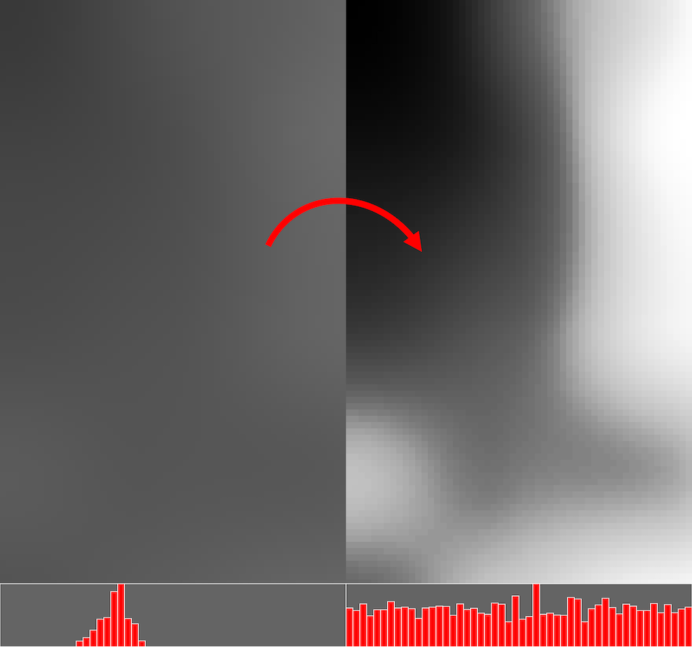
This is exactly the technique I used in Hoopla for the Equalized Flow (right) option of the Colour method param, compared to raw flow option (left) below:

That’s it! There are a few other ways that I’ve used histogram equalization beyond colour palette mapping, and I’m sure there are many more applications that I’ve not thought of.

I hope you find this technique useful in your future projects!

You can find the full code and a tutorial corresponding to the above on my OpenProcessing profile.