Making Störungen
written by un_erscore
The initial premise for this work was to take a simple, perfect form and twist and deform it in ways that make it both vastly different, but still recognizable. It is a commentary on the beauty of perfect and imperfect forms resultant from small, cumulative, and incremental changes. The butterfly effect in motion.
Creating the perfect form
The first step in this process is to create our perfect form, the canvas upon which our perturbations will be painted. I wanted the basis for this perfect form to both fill the space fully as well as be a single line, so for these criteria, a spiral made the most sense.
Accomplishing this is relatively simple. Create a walker class that determines the parameters required to draw a spiral and then draw it outward step by step.
const walker = {
  drawing: true,
  pos: new Vec2(0, 0),
  radius: 1000,          // the radius of the spiral
  coilsize: 3,           // The distance between coils
  stepSize: 3,           // The Size of each step
  coils: null,           // The number of rotations in the spiral
  thetaMax: null,        // The full distance travelled in radians
  stepTheta: null,       // How far to step away for each side
  theta: null,           // The current angle of the spiral
  steps: 0,
  origin: new Vec2(w / 2, h / 2),
  // Initialise our values
  init: function() {
    this.coils = this.radius / this.coilsize;      // The number of coils the spiral will have
    this.thetaMax = this.coils * 2 * Math.PI;      // The maximum value that theta can get to before escape
    this.stepTheta = this.radius / this.thetaMax;  // Theta stepsize
    this.theta = this.stepSize / this.stepTheta;   // The initial theta value
  },
  walk: function() {

    // If the radius has reached it's maximum, we stop drawing.
    if(this.theta > this.thetaMax) this.drawing = false;

    // The distance of this step from the center
    // Calculated by multiplying the angular step size by the current theta
    let distance = this.stepTheta * this.theta;

    // Straight up spiral - polar coordinates
    let p = new Vec2(distance, this.theta);

    // Update the theta by the stepSize / distance
    this.theta += this.stepSize / distance;

    // Creat our output cartesian coordinates
    const cart = polarToCartesian(p);

    this.steps++;

    // Finally, plot
    this.plot(cart);
  },

  }
}
We also need a way to translate to and from polar coordinates, this is a simple thing.
const cartesianToPolar = (p) => {
  return new Vec2(
    Math.hypot(p.x, p.y),
    Math.atan2(p.y, p.x)
  );
}
const polarToCartesian = (p) => {
  return new Vec2(
    Math.cos(p.y) * p.x,
    Math.sin(p.y) * p.x
  );
}
The result? An Archimedean spiral. (https://openprocessing.org/sketch/1671394)
Before moving onto the next major step, I also wanted to make sure that our final output is plottable, so to make sure that we're not drawing any lines outside of the boundaries of our piece, we can do this by introducing this code before our plot command.
if(
  cart.x < -this.origin.x + 10. ||
  cart.x > this.origin.x - 10. ||
  cart.y < -this.origin.y + 10. ||
  cart.y > this.origin.y - 10. ||
  this.steps <= 2
) return this.pos = cart;
Some simple perturbations
The next step in the process was to introduce some simple perturbations. These are trigonometric functions that are used to deform the spiral as it travels around its path. The idea with these is that they perform some small nudging of the walker's position as it moves, these small nudges accumulate and become more and more pronounced over time. Here is a basic function and the result that it produces.
{
  const cart = polarToCartesian(p);
  const cx = cart.x / 30;
  const cy = cart.y / 30 + 1.5;

  cart.x += (cos(cy)) * 30;
  cart.y += (sin(cx)) * 30;

  p = cartesianToPolar(cart);
}
(https://openprocessing.org/sketch/1671410)
From there it was a matter of playing with playing with further trigonometric perturbations until a library was built up. Here's another example:
{
  const cart = polarToCartesian(p);
  const cx = cart.x / 20 + 1.5;
  const cy = cart.y / 20 - 3.5;

  cart.x += cos(cy) * cos(cx) * 15;
  cart.y += (sin(cx) - sin(cy)) * 15;

  p = cartesianToPolar(cart);
}
(https://openprocessing.org/sketch/1672270)
Layering perturbations
One of the nice things about working with these sorts of fundamental functions is that they can be layered on top of each other. Consider the following, which comprises of the two functions I have previous illustrated, and you can clearly see in the image that this is the sum of the two functions, but that it has produced something new.
{
  const cart = polarToCartesian(p);
  let cx = cart.x / 20;
  let cy = cart.y / 20;

  cart.x += cos(cy) * cos(cx) * 15;
  cart.y += (sin(cx) - sin(cy)) * 15;

  cx = cart.x / 20;
  cy = cart.y / 20;

  cart.x += cos(cy) * 20;
  cart.y += sin(cx) * 20;

  p = cartesianToPolar(cart);
}
(https://openprocessing.org/sketch/1672311)
Generalizing the perturbations
This was the more difficult part, creating a structure that could adequately describe any perturbation function I could provide. This was necessary because the final token would have a variable number of very random perturbations, and so I needed to create a language to do so. The first part of doing so was to break the functions down into their different components. This was relatively easy as the components consist of, broadly speaking, variables and components.
{
  const cart = polarToCartesian(p);

  // THESE ARE THE VARIABLES
  const cx = cart.x / 20;
  const cy = cart.y / 20;

  // THESE ARE THE COMPONENTS
  cart.x += cos(cy) * cos(cx) * 15;
  cart.y += (sin(cx) - sin(cy)) * 15;

  p = cartesianToPolar(cart);
}
I decided early on that the easiest way to accomplish such a generalization was to provide a simple string syntax that would be parsed using regexp and the JavaScript function constructor, which allows you to provide a string that comprises the body of the function - N.B. this is a safer way to run eval on strings, but is still not entirely safe, use at your own risk.
This first block of code represents the generalization of the variables component.
/* This function provides a afacility with allows the operands to
 * pass back into the variables or components. It does this by
 * looking for any variable name with an _ in front of it and
 * replacing that with an `operands` property.
 */
const replaceOperands = (op, operands) => {
  for (let i in operands) {
    op = op.replaceAll(`_${i}`, `operands.${i}`);
  }
  return op;
};

// sc is the factor by which the cartesian components are divided
const sc = 10;
// The cartesian components. In the program, this would be replaced with a dynamic value
const cart = { x: 10, y: 10 };

// The operands object that will end up carrying all of the variables (including the loopbacks)
let operands = {};

/* The variable components. Each of these will be executed in order
 * You can see, in the last item, a demonstration of the loop back:
 * `c = _a / sc`, that _a will evaluate to `operands.a`, so if
 * `sc = 10` and `cart.x = 10`, this property will evaluate to `c = 0.1`
 */
const q = ["a = cart.x / sc", "b = cart.y / sc", "c = _a / sc"];

// Loop through all of the components and execute
for (let i = 0, o = q[i]; i < q.length; o = q[++i]) {
  // Find the variable name. a, b, c as above.
  const it = /(\w+)+/.exec(o)[1];
  // Replace any operand directives in the components
  const ops = replaceOperands(/.*=\s*(.+)/.exec(o)[1], operands);
  console.log(ops);
  /* This is where the magic happens. Take the variable string
   * and turn it into a function string that is immediately
   * executed with the operational components. Because this
   * executes in explicit order, previous components are passed
   * back into these functions as operands.
   */
  operands[it] = Function(
    `return function(cart, sc, operands) { return ${ops} }`
  )()(cart, sc, operands);
}

console.log(operands);
From here, I needed to codify and operate on the components part of the function. This is the part that changes the content on the resultant vector.
// Represents the amplitude of the function as applied to the component
const f = 20;

/* The components. These will execute on the provided cartesian
 * coordinates ad well as beig passed back into the operands
 * object for further processing, if necessary.
 */
const r = ["x += cos(_a) * f", "y += sin(_b) * f"];

// Loop through all of the components and execute
for (let i = 0, o = r[i]; i < r.length; o = r[++i]) {
  // The variable name, x, y etc.
  const it = /(\w)+/.exec(o)[1];
  // Separated out the various components of the function
  const ops = /.*(.=)\s*(.+)/.exec(o);
  // Builds the name of the component within the vector
  const prop = `cart.${it}`;
  // The method, +=, -= etc.
  let method = ops[1];
  // The replaced operands
  let op = replaceOperands(ops[2], operands);
  console.log(
    `return function(cart, operands, sc, f) { const os = (${op})*sc; operands['_${it}'] = os; ${prop}${method}os; }`
  );
  /* The final function. As before, this creates and executes
   * a function, in this case it updates both the variable on
   * the vector **and* adds the component back into operands
   * in case you want to use it in further calculations.
   */
  Function(
    `return function(cart, operands, sc, f) { const os = (${op})*sc; operands['_${it}'] = os; ${prop}${method}os; }`
  )()(cart, operands, sc, f);
}
Phew, that's a lot, if you would like to see this in an isolated format where you can play around with the variables to see how it works see https://openprocessing.org/sketch/1672345
See the final token here https://www.fxhash.xyz/generative/19682