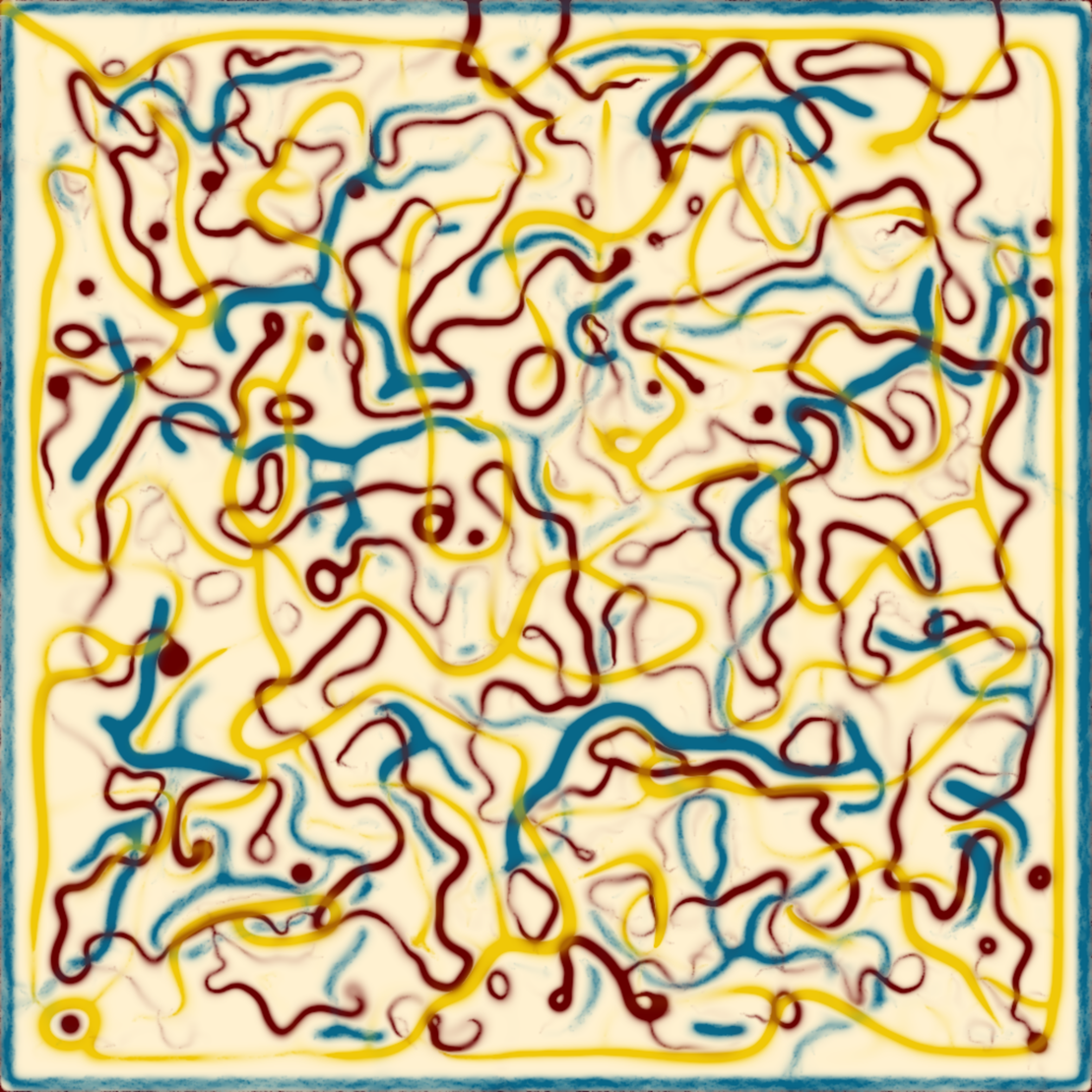
The core algorithm for 'follow my lead' is that of the Physarum slime mold - a model in which slime mold particles make their best effort to follow along in the path of other particles. I first came across this model some number of years ago in a post by Sage Jenson (http://cargocollective.com/sagejenson/physarum).

The basic idea behind the core algorithm is that you have a whole bunch of individual mold particles moving around in a 2d space. As they travel, they leave behind a chemical deposit. Over time, this substance decays and (potentially) diffuses outwards, leaving us with a chemical map showing where other physarum have recently been.

Physarum are equipped with three sensors that are able to process the concentration of the deposit in a particular location. One of these sensors is some distance directly in front of them, while the other two are offset to either side by some angle.

Each time step, the agent takes three readings (left, front and center), and then decides whether it wishes to continue on its current heading, or adjust by a fixed angle in either direction. For example, if the left sensor reading shows a higher concentration than both right and center, it may choose to adjust its heading leftwards.

This core model already leads to some interesting behaviors, and gives us a number of different settings we can play with, such as:

• how far away the three sensors are from the agent
• how far we move each time step
• what angle the two side sensors are offset from the center
• how much we change our heading when we rotate
• how much the chemical deposit decays over time
• whether or not the chemical deposit diffuses as it decays

I went on to extend this algorithm in a few different directions. The biggest change that I made was to run with three sets of physarum at a time, and to have each set be either indifferent towards each other group, or attracted/repulsed to some degree. In particular, I have a few starting regimes:

• Everyone is attracted to physarum of the same group, indifferent to one other group, and somewhat repulsed by the third group.
• Everyone is attracted to physarum of the same group, one pair of groups is somewhat repulsed by each other, and the final group is repulsed by both.
• Everyone is attracted to physarum of the same group and somewhat repulsed by all others.

However, with some low frequency, I allow these relationships to all become jumbled. The result is that in addition to its relationship with other groups, a group of physarum have a chance of being self-attracted, self-loathing, or self-indifferent.

There are two more ways that I created variability for this project. The simpler of these is to have some variability in where physarum particles begin their existence. Here the most common version is to have them randomly distributed across the entire 2d plane, but other options include having them start from a particular edge, from a circle, square, or line in the middle, from a diagonal, or based on a flow field.

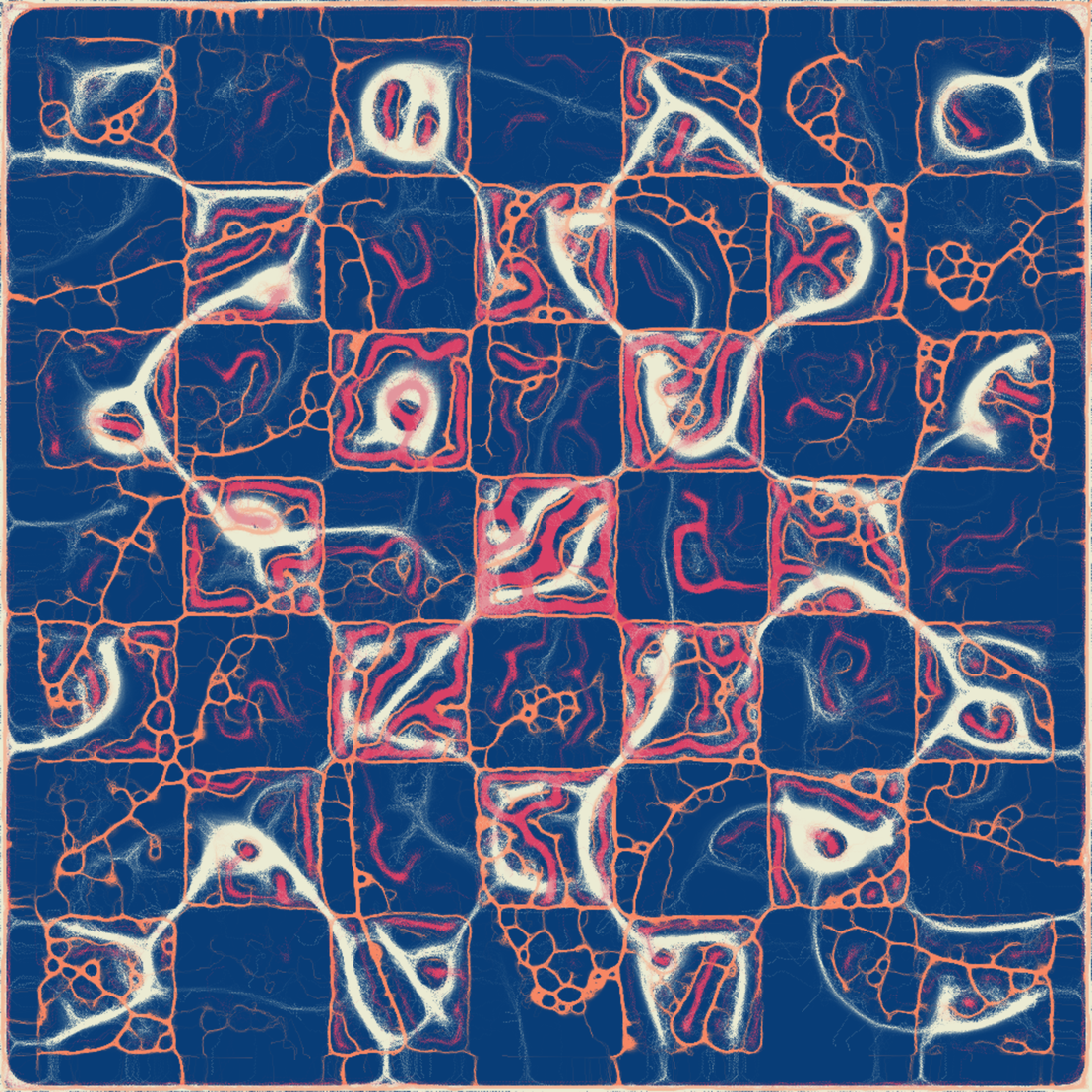
The other significant source of variability is in the creation of a landscape/height map. Essentially what I'm doing is saying that for each pixel in our 2d space, pretend that it in 3d space it exists at a particular height. Each group of phyasurm particles are then created with a preference for either moving uphill or downhill. When taking sensor readings, individuals now look at both the amount of chemical deposit and the height at each of their sensor locations, and combine that knowledge to make a decision about whether or not to update their heading.

There are a number of different ways these landscapes are created. For example 'grid' divides the space into a set of squares, and randomly assigns each a height. 'lines' just draws a couple of dividing lines onto our landscape. Landscapes also potentially include a border, which is just a gradient along the edges that discourages (or encourages) particles from travelling there.

Technical Details and Challenges

The remaining content is more on the technical side. Feel free to ignore everything beyond here if that's not your cup of tea. If you are interested, I've also shared all of the code in a github repo here. If you end up finding the code useful, please do let me know.

In general the set of steps taken in this project are:

1. Create all initial particle data (positions, headings, and other group specific settings)
2. Create a landscape/heightmap
3. Update particle positions/headings base on (a) particle's current position/heading (b) settings for the group this particle belongs to (c) landscape/heightmap (d) the trail map of chemical deposits
4. Create a representation of new chemical deposits based on particle positions
5. Update our trail map based on new deposits
6. Decay all exist deposits by some amount
7. Potentially diffuse chemicals
8. Repeat steps 3-7 300 times
9. Render the trail map of chemical deposits onto the screen

One of the biggest challenge to dealing with Physarum is the number of particles involved - we are generally running with somewhere between 60k and 160k particles in this project. This necessitates the user of shaders, where I have some knowledge, but am by no means an expert.

Initially, I didn't know how to use the GPU to both update agent positions/headings, and to deposit chemicals at those locations. Early versions had me doing the first step on the CPU and only using the GPU for drawing. This severely limited the number of particles I could run with and still have reasonable performance.

Then I found a different Physarum implementation here (https://github.com/amandaghassaei/gpu-io/blob/main/examples/physarum/index.js) that showed me how I could

• create a texture that contains agent pos/heading
• update pos/heading using a shader
• use the gl.POINTS primitive and gl_VertexID to create my chemical deposit using my agent texture

This meant that I could essentially have all logic running on the GPU using shaders. See `src/layers/deposit.ts' to see how I do this in my project.

Browser Differences

Another challenge that I ran into was in handling differences between different browsers. Initially I had been creating my landscapes using the canvas API. However, it turned out that there were a lot of ways that different browsers would draw things with very slight differences. For example, here are the lightness values after drawing a triangle in Firefox vs. in Chrome

The difference is exceptionally tiny, but the nature of this project is that these sorts of small changes can go on to have notable effects. Specifically, our Physarum particles are looking at gradients, so they tend to not to care only about relative values. Having two pixels be slightly different vs. identical can cause a particle to adjust it's heading and drop its next deposit on a different pixel. That change will cascade further down the line, as now we have both a landscape difference (because of browser differences) and a trail map difference (because the deposit happened at a different location).

In light of this, I decided to rewrite all of my landscapes using WebGL shaders, although that ended up having its own set of challenges.

Hardware/GPU Differences

When writing WebGL shaders, you're telling the computer exactly what should happen at each pixel. So instead of saying "draw a white rectangle whose top left corner is at (x,y) that has a width of w and a height of h," you say something along the lines of "if the current pixel's horizontal location is between x and x+w, and it's vertical location is between y and y+h, return the color 'white', otherwise return the color 'black'." This pixel level precision was exactly what I needed to solve my problems of different browsers behaving slightly differently.

The problem I ran into next was that when doing floating point math (i.e. math with non-integer values), different GPUs/hardware were not always generating the same results. My understanding is that this largely has to do with how they handle precision (side note: it is entirely possible that there are errors in my explanation below, but this is an attempt to share my mental model).

For example, the decimal representation of the fraction 2/9 is a zero, followed by a decimal point, followed by an infinite number of twos, i.e. 0.22222.... The computer does not have an unlimited amount of memory to store all of these twos, so it ends up storing a number that is necessarily less price. For example, it might choose to round it down after the 16th 2 and store it as 0.2222222222222222. One problem that we run into is that some hardware will have more or less room to store this value, so on another machine it choose to round it even sooner, say after the 8th two (0.22222222). This has the potential to change the result of other numbers that we calculate using this value.

The other problem is that even in cases where two machines have the identical storage, they might end up taking slightly different approaches to how to reduce precision. For example, both 1.1 and 1.2 are less precise versions of 1.15 with an equal amount of loss.

I ended up taking a few different strategies to mitigate this - I'm not certain how well advised any of them are.

float sin2(float radians) { 
  // go from radians to a 0-1 range
  float pctTau = mod(radians / TAU, 1.); 
  // figure out which of our 512 availabe buckets we want to be in
  pctTau = (floor(pctTau * 512.) + 0.5) / 512.; 
  // get the hard-coded sin value from the texture (y for cos value)
  return texture(u_sincos, vec2(pctTau, 0.)).x; 
}

The next strategy I took was to coarse grain my calculations in various places. Essentially, what I was doing was intentionally decreasing precision. An example of this is something like:

x = floor(x * 1000.)/1000.;

This makes it so that a number like 0.12311111 and 0.12322222 will both be treated as 0.123, leading to fewer opportunities for different hardware to get different results. Figuring out the "right" level of coarse graining was a lot of trial and error rather than being based on any sort of principled understanding. For this reason, I'm still not entirely convinced this approach is a good one.

My final mitigation was that in the case of my diffusion calculation, I made a point to do as much of my math as I could using integers instead of floating point values. This was again a way of reducing precision. What I do is read in a floating point value from a texture, multiply it by some large scaling factor (1024), do various adds and divides in integer space, then convert it back into a float, while dividing by the scaling factor. This ended up being quite successful, and fixed all of the discrepancies I'd been seeing in this layer. The one caveat was that I now needed to be careful to guard against integer overflows, particularly if my scaling factor was large. This code all lives in `src/layers/diffuse.ts'.

With these steps, I got to a point where I was consistently seeing pixel for pixel identical results across my three test devices (MacBook Pro, iPad, Linux with hardware acceleration disabled) as well as with the FxHash minter.

If you've made it this far, and missed the link halfway through this doc, all of the code for this project can be found at https://github.com/ArtOfGabriel/follow_my_lead_public